Spreadsheet Review Assignment
- Start a new spreadsheet. Starting in cell A4, enter about seven names going down the page (it is useful to enter the first and second names separately, in case we want to sort the spreadsheet by name later).
- In cells C1. El, GI, and I1 enter 'Test 1', 'Test 2', 'Essay', and 'Presentation' respectively. On the row below, each of these headings, enter 'Max mark' under each heading.
- Starting in cell C3, enter the headings 'Mark', then 'Percentage', repeating up to and including cell J3. In K3 enter 'Total'.
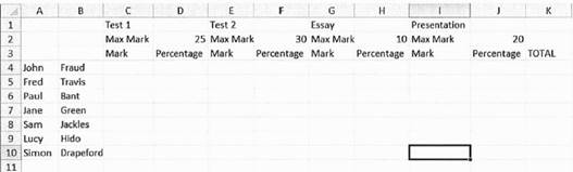
- Enter the following maximum marks for each assignment, starting in cell D2. Test 1 - 25; Test 2 - 30; Essay -10; Presentation - 20. Your spreadsheet should now look something like the screenshot below.
- Enter marks for each student for each assignment (make sure they are no higher than the maximum mark for each assignment).
- In D4, calculate the percentage for the first student's Test 1 grade. Calculate the percentages for each remaining assignment.
- If the formula in cell D4 is copied down to D5, strange things start to happen. This is because by default, the spreadsheet uses relative cell addressing - when you copy or paste a formula, the cell references in the formula are updated. So copying and pasting C4/D2*100 to the line below changes it to C5/D3*100, then C6/D4*'100, and so on.
- Sometimes relative cell addressing is useful. In this case, we do want the C4 to change to a C5, because we are looking at the next student's grade. However, we do not want D2 to change - for every student in this column, we want to divide the grade by D2. To achieve this we need to use absolute cell referencing, which is achieved with the dollar sign ($). Change the formula in cell D4 to read:
- The dollar sign says 'use absolute cell referencing for the number 2'. Copy and paste this formula down column D for each student.
- Calculate the percentage for each student for the remaining three assignments. Use absolute cell referencing where needed.
- Enter a formula in column K to calculate the total number of marks for each student (each assignment added together).
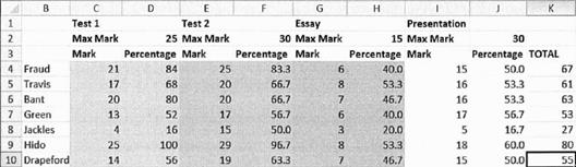
- Earlier, we made a mistake. The essay is actually out of 15 marks, not 10, and the presentation is out of 30. Change the appropriate cells in the spreadsheet (there should only be two of them). Notice how the percentages automatically recalculate themselves. Automatic recalculation is an important feature of spreadsheet software.
- Spreadsheets have some built in functions to help with common mathematical tasks. One such function is AVERAGE, which calculates the mathematical mean. AVERAGE is used with a cell range to specify the cells it will operate on. To calculate the average percentage for Test 1, enter the following in cell D11:
- The cell range tells the function to use the values of all cells from D4 to D10, inclusive. Using cell ranges is quicker and less error-prone than writing out each cell's reference (D4+D5+D6+D7+D8+D9+D10).
- If you copy cell D11 to cell F11, you will see that the correct average is calculated for column F. This is because relative cell referencing has been used, changing the function from AVERAGE(D4:D13) to AVERAGE(F4:F13) automatically.
- Other basic spreadsheet functions include MAX, MIN, SUM. Use MIN and MAX in appropriate cells to find the maximum and minimum grade for each assignment.
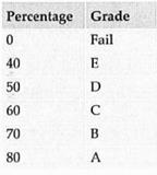 Starting in cell M15, enter the percentage and grade data in the table shown here.
- It would be really helpful if column L could contain a letter grade to go with the total percentage. The LOOKUP function can be used to achieve this. The lookup function accepts a cell value and a table of values. It looks up the value in the first column of the table (percentage in our case) and returns the corresponding value from the second column (the grade in our case). The percentages in the table above are the minimum for each grade (you must get at least 70% to get a B, 80% to get an A, etc.). In cell L4, enter:
=LOOKUP(K4,M$16:M$21,N$16:N$21)
- Note the use of absolute cell referencing when referring to the table. Copying and pasting this formula down column L should result in a letter grade for each student. If the grades are wrong, check that you used absolute cell referencing when writing the formula.
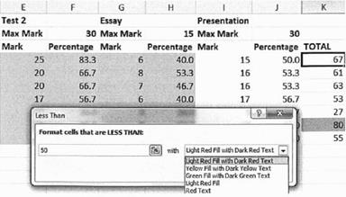 Use Conditional formatting to change the formatting of a cell based on its value. In this spreadsheet, it would be good to highlight students who are failing in red, and those who are doing particularly well in green. Apply conditional formatting twice to achieve these two goals.
- The COUNTIF function is used to count the number of cells which match a given criteria. Use COUNTIF in the column K to count the number of failed students. Display the results in any appropriate spot.
The percentage can be calculated by entering the
following formula: = C4/ D2 * 100
Note that you use a cell reference rather than the number itself.
=C4/D$2*100
=AVERAGE(D4:D10)
Alternative
In OpenOffice or LibreOffice, instead use: =LOOKUP(K4,M$16:M$21,N$16:N$21)